Point Transformer 论文

BinaryOracle2025/8/31大约 33 分钟约 9829 字

Point Transformer 论文

论文: Point Transformer
代码: https://github.com/POSTECH-CVLab/point-transformer

引言

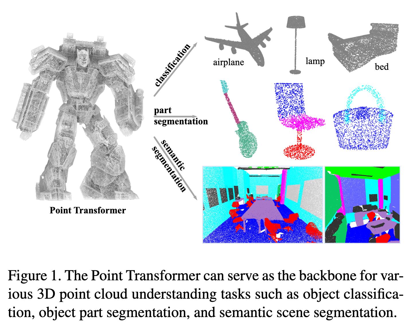
背景与动机（如图1所示）：

3D 点云广泛存在于自动驾驶、增强现实和机器人等应用中，但它们与图像不同，是嵌入在连续空间的集合，因此传统基于卷积的视觉网络难以直接应用。
现有方法主要有三类：
- 将点云体素化后应用 3D 离散卷积，但计算和内存开销大，并未充分利用点云稀疏性。
- 使用稀疏卷积、池化或连续卷积直接在点上操作，部分缓解了计算负担。
- 将点集构建成图结构，通过消息传递进行信息传播。
Transformer 的自注意力机制天然适合点云，因为它对输入的排列和数量不敏感，而点云本质上就是集合结构。

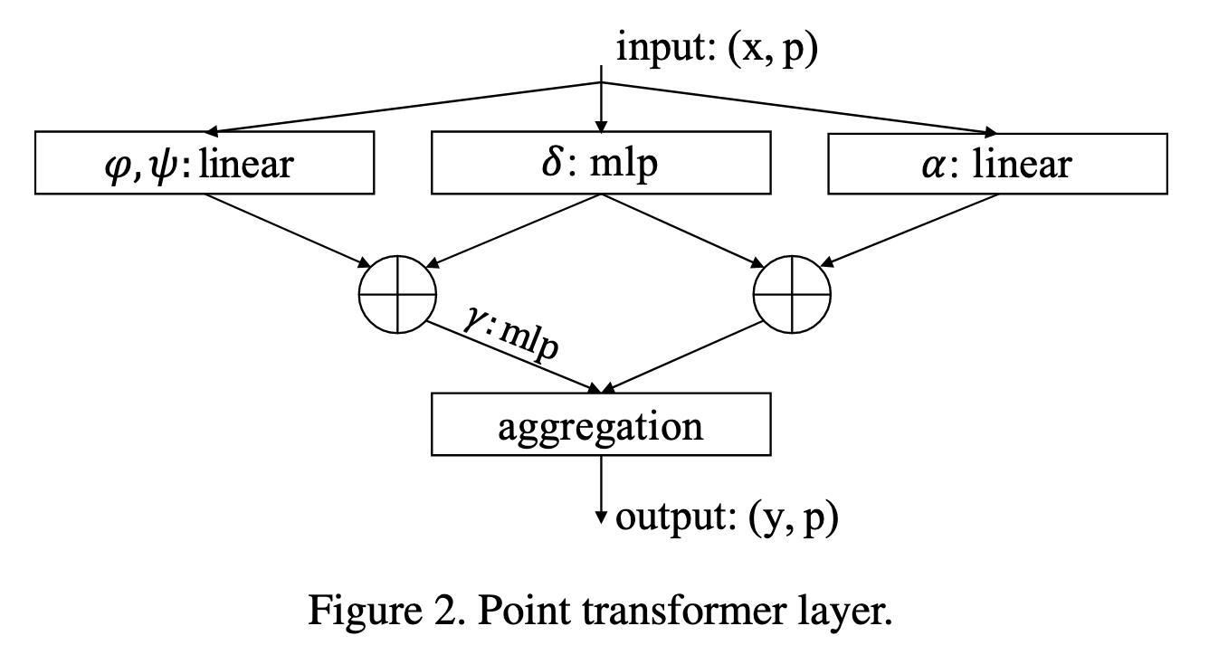
方法设计（如图2所示）：

我们提出了 Point Transformer 层，能够处理点云的排列和数量不变性，通过局部邻域的自注意力传播信息。
在网络设计上，完全由自注意力和逐点操作组成，不依赖卷积操作，也不需要事先体素化。
通过对自注意力算子形式、局部邻域应用方式及位置编码方法的设计，构建了高表达能力的网络骨干，可用于多种 3D 理解任务。

主要贡献：

设计了高度表达能力的 Point Transformer 层，本质上适合点云处理，对排列和数量不敏感。
构建了基于 Point Transformer 层的高性能网络，可作为 3D 场景理解的通用骨干，适用于分类和密集预测任务。
在多个领域和数据集上进行了广泛实验，创下多个最先进水平，超越大量先前方法。

方法

背景

Transformer 和自注意力在 NLP 和图像分析中已经非常成功。自注意力分为两种：标量注意力和向量注意力。

标量注意力
输入是一组特征向量 $X = x_{i}$ ，输出 $y_{i}$ 的计算公式为：
$y_{i} = \sum_{x_{j} \in X} ρ (ϕ (x_{i})^{⊤} ψ (x_{j}) + δ) α (x_{j})$
其中 $ϕ, ψ, α$ 是点级特征变换（线性投影或 MLP）， $δ$ 是位置编码， $ρ$ 是归一化（如 softmax）。注意力权重是标量。
向量注意力
注意力权重是向量，可以对不同通道单独调制，计算方式为：
$y_{i} = \sum_{x_{j} \in X} ρ (γ (β (ϕ (x_{i}), ψ (x_{j})) + δ)) ⊙ α (x_{j})$
其中 $β$ 是关系函数（如减法）， $γ$ 是生成向量权重的 MLP。

这两类自注意力算子本质上都是集合算子，既可以在整个集合上作用（如句子、整幅图像），也可以只在局部子集上作用（如图像 patch）。

Point Transformer 层

点云天然就是不规则的集合，因此自注意力特别适合点云。Point Transformer 层基于向量自注意力，采用减法关系并在注意力分支和特征分支都加入位置编码：

y_{i} = \sum_{x_{j} \in X^{(i)}} ρ (γ (ϕ (x_{i}) - ψ (x_{j}) + δ)) ⊙ α (x_{j}) + δ

其中 $X^{(i)}$ 是 $x_{i}$ 的 $k$ 近邻集合（局部邻域）。映射函数 $γ$ 是一个两层线性层 + ReLU 的 MLP。结构如图2所示。

位置编码

位置编码让注意力能够感知局部空间结构。

在 NLP/图像中，常用正弦余弦或归一化坐标范围手工设计。
在 3D 点云中，点的坐标天然可用作位置编码。

本文提出 可训练的参数化位置编码：

δ = θ (p_{i} - p_{j})

其中 $θ$ 是一个两层线性层 + ReLU 的 MLP。

实验发现，位置编码对注意力生成分支和特征变换分支都很重要，因此在公式 (3) 的两个分支中都加了 $δ$ 。 $θ$ 与整个网络一起端到端训练。

Point Transformer 模块

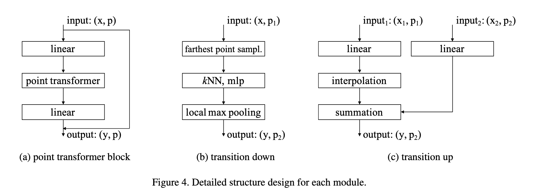
Point Transformer 模块是一个残差结构，如图4(a) 所示。它包含：

Point Transformer 层（核心）
降维的线性投影（加速计算）
残差连接

输入是一组点的特征向量及其 3D 坐标，输出是更新后的点特征。该模块在特征内容和三维空间布局上都能自适应进行信息聚合。

网络架构

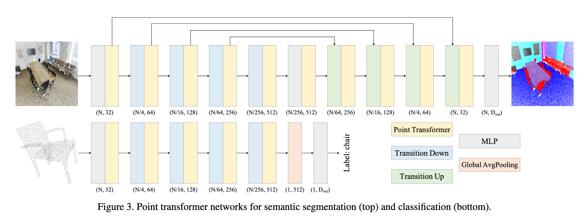
整个网络完全由 Point Transformer 模块、点级变换和池化组成，不依赖卷积。结构如图3所示。

骨干网络结构：

语义分割/分类的特征编码器有 5 个阶段，下采样率为 $[1, 4, 4, 4, 4]$ ，输出点数依次为 $[N, N / 4, N / 16, N / 64, N / 256]$ 。相邻阶段通过转换模块连接：

Transition down（图4b）：
从 $P_{1}$ 采样子集 $P_{2}$ （最远点采样），并将 $P_{1}$ 的特征汇聚到 $P_{2}$ 。流程：
- 线性层 → BN → ReLU
- kNN 聚合（ $k = 16$ ）
- max pooling
Transition up（图4c）：
在解码阶段，将 $P_{2}$ 的特征映射回更高分辨率点集 $P_{1}$ ：
- 线性层 → BN → ReLU
- 三线性插值
- 融合来自编码器的跳跃连接特征

输出头：

语义分割：为每个点生成特征 → MLP → 每点分类 logits
分类任务：对点特征全局平均池化 → 全局特征向量 → MLP → 分类 logits

消融实验

为了验证 Point Transformer 设计中的关键选择，作者进行了多组消融实验，结果如下：

邻居数量 k 的影响：

当 $k = 16$ 时性能最佳。
当 $k = 4$ 或 $k = 8$ 时，邻域过小，缺乏足够上下文，导致预测不准确。
当 $k = 32$ 或 $k = 64$ 时，邻域过大，引入过多不相关点，噪声增加，反而降低性能。

Softmax 正则化的作用：

不使用 Softmax 时，mIoU/mAcc/OA = 66.5% / 72.8% / 89.3%。
使用 Softmax 时，性能显著提升至 70.4% / 76.5% / 90.8%。
结论：Softmax 归一化是必要的，否则模型性能显著下降。

位置编码 δ 的选择：

无位置编码 → 性能明显下降。
使用绝对位置编码 → 性能有所提升。
使用相对位置编码 → 性能最佳。
仅在注意力生成分支或特征变换分支单独加入相对位置编码 → 性能下降。
结论：必须在两条分支同时加入相对位置编码，效果最好。

注意力类型的比较：

MLP：逐点 MLP，无邻域交互，性能最差。
MLP+pooling：逐点 MLP + 邻域池化，有信息交互但无注意力机制，性能优于纯 MLP。
标量注意力：基于公式 (1)，比前两者更强。
向量注意力：基于公式 (3)，性能最优。
实验结果显示，标量注意力的 mIoU 为 64.6%，而向量注意力达到 70.4%，提升 5.8 个百分点。
结论：向量注意力由于支持逐通道自适应调制，表达能力更强，对 3D 数据处理尤为有利。

代码实现

向量自注意力层

PointTransformerLayer 类实现了Point Transformer论文中提出的向量自注意力机制，该机制是点云处理领域的重要创新。与传统的标量注意力不同，向量注意力能够更好地捕获3D空间中的几何关系。

核心设计理念：

向量化注意力：注意力权重不再是标量，而是向量形式，能够编码更丰富的空间信息
位置感知：通过位置编码函数θ将3D相对坐标信息融入注意力计算
局部邻域处理：基于KNN构建的局部邻域，实现高效的点云特征聚合

算法流程概述：

特征变换：将输入特征通过线性层生成Q、K、V三元组
邻域构建：利用KNN算法为每个点构建局部邻域
位置编码：将相对坐标通过MLP网络映射到高维特征空间
注意力计算：结合特征差值和位置编码生成向量化注意力权重
特征聚合：基于注意力权重对邻域特征进行加权融合

完整的向量自注意力计算代码实现如下：

class PointTransformerLayer(nn.Module):
    def __init__(self, in_planes, out_planes, share_planes=8, nsample=16):
        super().__init__()
        # 中间通道数，简化处理（这里直接等于 out_planes）
        self.mid_planes = mid_planes = out_planes // 1
        self.out_planes = out_planes
        self.share_planes = share_planes
        self.nsample = nsample

        # Q, K, V 的线性变换
        self.linear_q = nn.Linear(in_planes, mid_planes)   # 查询向量 (query)
        self.linear_k = nn.Linear(in_planes, mid_planes)   # 键向量 (key)
        self.linear_v = nn.Linear(in_planes, out_planes)   # 值向量 (value)

        # 位置编码 δ (论文 Eq.(4): δ = θ(pi − pj))
        # 输入是相对坐标 (3D)，输出是与 out_planes 对齐的特征
        self.linear_p = nn.Sequential(
            nn.Linear(3, 3),
            nn.BatchNorm1d(3),
            nn.ReLU(inplace=True),
            nn.Linear(3, out_planes)
        )

        # 权重生成函数 γ (MLP)，作用在 (q - k + δ) 上
        # 注意这里做了“通道分组”（share_planes），减少计算量
        self.linear_w = nn.Sequential(
            nn.BatchNorm1d(mid_planes),
            nn.ReLU(inplace=True),
            nn.Linear(mid_planes, mid_planes // share_planes),
            nn.BatchNorm1d(mid_planes // share_planes),
            nn.ReLU(inplace=True),
            nn.Linear(mid_planes // share_planes, out_planes // share_planes)
        )

        # softmax 用来对注意力权重归一化
        self.softmax = nn.Softmax(dim=1)

    def forward(self, pxo) -> torch.Tensor:
        # 输入:
        # p: 点的坐标 (n, 3)
        # x: 点的特征 (n, c)
        # o: batch 索引 (b)
        p, x, o = pxo

        # 得到 Q, K, V
        x_q, x_k, x_v = self.linear_q(x), self.linear_k(x), self.linear_v(x)  # (n, c)

        # 构建邻域 (kNN)，并返回局部邻域的特征
        # x_k: (n, nsample, 3+c)，包含相对坐标和 K 特征
        # x_v: (n, nsample, c)，邻域内的 V 特征
        x_k = pointops.queryandgroup(self.nsample, p, p, x_k, None, o, o, use_xyz=True)
        x_v = pointops.queryandgroup(self.nsample, p, p, x_v, None, o, o, use_xyz=False)

        # 分离相对坐标 p_r 和邻域内的 K 特征
        p_r, x_k = x_k[:, :, 0:3], x_k[:, :, 3:]

        # 将相对坐标 p_r 输入位置编码 MLP θ
        # 这里因为 BatchNorm 的维度问题，需要转置 (n, nsample, 3) ↔ (n, 3, nsample)
        for i, layer in enumerate(self.linear_p):
            p_r = layer(p_r.transpose(1, 2).contiguous()).transpose(1, 2).contiguous() if i == 1 else layer(p_r)
        # 经过 MLP 后: (n, nsample, out_planes)

        # 根据 Eq.(3): w = γ(φ(xi) − ψ(xj) + δ)
        # x_q.unsqueeze(1): (n, 1, c)，与邻域对齐
        # p_r reshape 后与 x_k 对齐做相加
        w = x_k - x_q.unsqueeze(1) + p_r.view(
            p_r.shape[0], p_r.shape[1], self.out_planes // self.mid_planes, self.mid_planes
        ).sum(2)  # (n, nsample, c)

        # 将 w 输入 γ MLP (linear_w)，得到注意力权重
        for i, layer in enumerate(self.linear_w):
            w = layer(w.transpose(1, 2).contiguous()).transpose(1, 2).contiguous() if i % 3 == 0 else layer(w)

        # softmax 归一化注意力权重
        w = self.softmax(w)  # (n, nsample, c)

        # 最终聚合 (Eq.(3) 中 ρ(...)*α(xj+δ))
        n, nsample, c = x_v.shape
        s = self.share_planes
        x = ((x_v + p_r).view(n, nsample, s, c // s) * w.unsqueeze(2)).sum(1).view(n, c)

        return x

下面针对上面部分代码进行进一步说明:

计算注意力权重: 领域内最近邻键特征 - 领域所在中心点查询特征 + 相对位置编码(巧妙的view方式，个人理解是为了确保维度对齐)

        w = x_k - x_q.unsqueeze(1) + p_r.view(
            p_r.shape[0], p_r.shape[1], self.out_planes // self.mid_planes, self.mid_planes
        ).sum(2)  # (n, nsample, c)

聚合: 对每个中心点的所有邻居点的特征在特征维度上进行分组，做通道分组(类似多头注意力，但是作用不完全相同) + 利用广播后做逐元素相乘，完成对同一个邻居点的所有通道分组应用相同权重分配的过程 + 所有邻居点特征进行求和，完成领域值信息聚合过程 + 多头重组回原貌

    # （200，8，8，4） * （200，8，1，4） -> (200, 8, 8, 4) -> (200,8,4) -> (200,32)
    x = ((x_v + p_r).view(n, nsample, s, c // s) * w.unsqueeze(2)).sum(1).view(n, c)

分组计算过程可参考如下这个简化版例子:

# 分组后的特征 (1个点，1个邻居，2组，每组2个通道)
grouped_features = torch.tensor([[
    [[1.0, 2.0],    # 组0: 通道0,1
     [3.0, 4.0]]    # 组1: 通道2,3
]])  # shape: (1, 1, 2, 2)

# 注意力权重 (16维权重，这里简化为2维)
attention_weights = torch.tensor([[
    [[0.5, 1.0]]    # 权重向量
]])  # shape: (1, 1, 1, 2)

# 逐元素相乘
result = grouped_features * attention_weights
# [[[[1.0*0.5, 2.0*1.0],   # 组0: [0.5, 2.0]
#    [3.0*0.5, 4.0*1.0]]]] # 组1: [1.5, 4.0]

这实际上是一种分组通道注意力（Grouped Channel Attention）：

不是在序列维度上做注意力（token-token）
而是在通道维度上做注意力（channel-channel）
通过分组实现参数共享

queryandgroup 方法实现了点云的邻域查询和特征分组功能。具体流程如下：

邻域查询：对于查询点集合中的每个点，利用 KNN 算法在所有点集合中寻找最近的 nsample 个邻居点，并返回这些邻居点的索引；
相对坐标计算：将每个查询点的邻居点坐标减去查询点自身坐标，得到以查询点为原点的局部相对坐标系；
特征分组：根据邻居点索引，提取对应的特征向量，形成每个查询点的邻域特征集合。

该方法的核心作用是将无序的点云数据转换为有序的局部邻域结构，为后续的注意力计算提供空间上下文信息。完整代码实现如下所示:

def queryandgroup(nsample, xyz, new_xyz, feat, idx, offset, new_offset, use_xyz=True):
    """
    查询并分组函数：为每个查询点找到最近邻并分组其特征
    input:
        nsample: 最近邻数量
        xyz: 所有点的坐标 (n, 3)
        new_xyz: 查询点的坐标 (m, 3)
        feat: 所有点的特征 (n, c)
        idx: 预计算的最近邻索引，如果为None则重新计算
        offset: 每个batch的点的结束索引 (b)
        new_offset: 每个batch的查询点的结束索引 (b)
        use_xyz: 是否在输出中包含相对坐标信息
    output:
        new_feat: 分组后的特征，如果use_xyz=True则为(m, nsample, 3+c)，否则为(m, nsample, c)
        grouped_idx: 分组后的索引 (m, nsample)
    """
    assert xyz.is_contiguous() and new_xyz.is_contiguous() and feat.is_contiguous()

    # 如果没有指定查询点，则使用所有点作为查询点
    if new_xyz is None:
        new_xyz = xyz

    # 如果没有提供预计算的索引，则调用KNN查询函数计算
    if idx is None:
        idx, _ = knnquery(nsample, xyz, new_xyz, offset, new_offset)  # (m, nsample)

    n, m, c = xyz.shape[0], new_xyz.shape[0], feat.shape[1]

    # 根据索引分组坐标：获取每个查询点的邻居坐标
    grouped_xyz = xyz[idx.view(-1).long(), :].view(m, nsample, 3)  # (m, nsample, 3)

    # 计算相对坐标：邻居坐标减去查询点坐标（局部坐标系）： （200，8，3） -  （200，1，3）= （ 200,8,3 ）
    grouped_xyz -= new_xyz.unsqueeze(1)  # (m, nsample, 3)

    # 根据索引分组特征：获取每个查询点的邻居特征
    grouped_feat = feat[idx.view(-1).long(), :].view(m, nsample, c)  # (m, nsample, c)

    # 根据use_xyz标志决定输出格式
    if use_xyz:
        # 拼接相对坐标和特征：输出形状为(m, nsample, 3+c)
        return torch.cat((grouped_xyz, grouped_feat), -1)
    else:
        # 只返回特征：输出形状为(m, nsample, c)
        return grouped_feat

KNNQuery 类实现了K近邻查询算法，其主要功能是为每个查询点寻找最近的邻居点。具体实现包含以下几个关键步骤：

1. 问题背景：在批处理点云数据时，不同样本的点云可能包含不同数量的点（如第一个点云1024个点，第二个点云2048个点），因此需要使用 offset 和 new_offset 参数来标记每个batch中点云的边界范围。

2. 算法流程：

对于每个查询点，计算其与当前batch内所有候选点的欧几里得距离
使用 torch.topk 函数选出距离最小的 nsample 个点
返回最近邻点的索引和对应的距离值

3. 实现特点：采用批处理方式提高计算效率，同时处理点云数量不一致的情况。完整代码实现如下:

class KNNQuery(Function):
    @staticmethod
    def forward(ctx, nsample, xyz, new_xyz, offset, new_offset):
        """
        KNN查询的前向传播函数
        input:
            nsample: 需要查询的最近邻数量
            xyz: 所有点的坐标 (n, 3)
            new_xyz: 查询点的坐标 (m, 3)，如果为None则使用xyz
            offset: 每个batch的点的结束索引 (b)
            new_offset: 每个batch的查询点的结束索引 (b)
        output:
            idx: 每个查询点的最近邻点索引 (m, nsample)
            dist2: 每个查询点到最近邻点的平方距离 (m, nsample)
        """
        if new_xyz is None:
            new_xyz = xyz  # 如果没有指定查询点，则对所有点进行自查询
        assert xyz.is_contiguous() and new_xyz.is_contiguous()
        m = new_xyz.shape[0]  # 查询点的数量

        # 初始化输出张量：索引矩阵和距离矩阵
        idx = torch.zeros((m, nsample), dtype=torch.long)
        dist2 = torch.zeros((m, nsample))

        # 按batch处理数据
        start_idx, new_start_idx = 0, 0  # 当前batch的起始索引
        for i in range(len(offset)):
            # 计算当前batch的结束索引
            end_idx = offset[i] if i < len(offset) else xyz.shape[0]
            new_end_idx = new_offset[i] if i < len(new_offset) else m

            # 确保当前batch有数据需要处理
            if end_idx > start_idx and new_end_idx > new_start_idx:
                # 提取当前batch的点坐标和查询点坐标
                batch_xyz = xyz[start_idx:end_idx]
                batch_new_xyz = new_xyz[new_start_idx:new_end_idx]

                # 计算查询点与所有点之间的欧几里得距离平方
                # 使用广播机制计算坐标差: (1,n,3) - (m,1,3) = (m,n,3) - (m,n,3) = (m_batch, n_batch, 3)
                diff = batch_xyz.unsqueeze(0) - batch_new_xyz.unsqueeze(1)  
                # (m_batch, n_batch) - 平方距离矩阵
                distances = torch.sum(diff ** 2, dim=-1)

                # 获取k个最近邻的索引和距离
                actual_nsample = min(nsample, distances.shape[1])  # 实际可用的最近邻数量
                # torch.topk返回最小的k个值及其索引: (m_batch,actual_nsample)
                knn_dist, knn_idx = torch.topk(distances, actual_nsample, dim=1, largest=False)

                # 如果实际邻居数量小于要求的nsample，进行填充
                if actual_nsample < nsample:
                    # 使用0填充索引和距离矩阵
                    padding = torch.zeros((knn_idx.shape[0], nsample - actual_nsample), dtype=knn_idx.dtype)
                    knn_idx = torch.cat([knn_idx, padding], dim=1)
                    knn_dist = torch.cat(
                        [knn_dist, torch.zeros((knn_dist.shape[0], nsample - actual_nsample), dtype=knn_dist.dtype)],
                        dim=1)

                # 将当前batch的结果存入总输出中，注意加上全局偏移量
                idx[new_start_idx:new_end_idx] = knn_idx + start_idx
                dist2[new_start_idx:new_end_idx] = knn_dist

            # 更新下一个batch的起始索引
            start_idx, new_start_idx = end_idx, new_end_idx

        # 返回最近邻索引和实际距离（加上小常数避免数值不稳定）
        return idx, torch.sqrt(dist2 + 1e-8)

Point Transformer 残差块

PointTransformerBlock 类是 Point Transformer 残差块，是 Point Transformer 架构中的基本构建模块 , 其代码实现如下所示:

class PointTransformerBlock(nn.Module):
    """
    Point Transformer 残差块
    实现预激活（Pre-Activation）的残差连接结构
    """
    expansion = 1  # 维度扩展系数，1表示输出维度与输入维度相同

    def __init__(self, in_planes, planes, share_planes=8, nsample=16):
        """
        初始化函数
        Args:
            in_planes: 输入特征维度
            planes: 中间特征维度（也是输出维度，因为expansion=1）
            share_planes: 通道分组数，用于减少计算量
            nsample: 每个点的邻居数量，用于kNN搜索
        """
        super(PointTransformerBlock, self).__init__()
        
        # 第一层：线性变换 + 批归一化（升维或保持维度）
        self.linear1 = nn.Linear(in_planes, planes, bias=False)  # 无偏置，因为后面有BN
        self.bn1 = nn.BatchNorm1d(planes)  # 批归一化，加速训练
        
        # 核心：Point Transformer 自注意力层
        self.transformer2 = PointTransformerLayer(planes, planes, share_planes, nsample)
        self.bn2 = nn.BatchNorm1d(planes)  # Transformer后的批归一化
        
        # 第三层：线性变换 + 批归一化（调整到最终输出维度）
        self.linear3 = nn.Linear(planes, planes * self.expansion, bias=False)
        self.bn3 = nn.BatchNorm1d(planes * self.expansion)  # 最终批归一化
        
        # 激活函数（原地操作节省内存）
        self.relu = nn.ReLU(inplace=True)
        
        # 注意：这里应该有残差连接的shortcut处理
        # 如果 in_planes != planes * expansion，需要投影层
        if in_planes != planes * self.expansion:
            self.shortcut = nn.Sequential(
                nn.Linear(in_planes, planes * self.expansion, bias=False),
                nn.BatchNorm1d(planes * self.expansion)
            )
        else:
            self.shortcut = nn.Identity()  # 恒等映射

    def forward(self, pxo):
        """
        前向传播
        Args:
            pxo: 元组 (p, x, o)
                p: 点坐标，形状 (n, 3)
                x: 点特征，形状 (n, in_planes)  
                o: 批次索引，形状 (b)
        Returns:
            元组 (p, x, o): 变换后的点坐标、特征和批次索引
        """
        p, x, o = pxo  # 解包：点坐标, 点特征, batch索引
        
        # 保存原始输入用于残差连接（需要处理维度匹配）
        identity = x
        
        # 第一层：线性变换 → BN → ReLU
        x = self.linear1(x)      # (n, in_planes) → (n, planes)
        x = self.bn1(x)          # 批归一化
        x = self.relu(x)         # ReLU激活
        
        # 第二层：Point Transformer 自注意力 → BN → ReLU
        x = self.transformer2([p, x, o])  # 应用自注意力，形状 (n, planes)
        x = self.bn2(x)          # 批归一化
        x = self.relu(x)         # ReLU激活
        
        # 第三层：线性变换 → BN
        x = self.linear3(x)      # (n, planes) → (n, planes * expansion)
        x = self.bn3(x)          # 最终批归一化
        
        # 残差连接：处理维度匹配问题
        identity = self.shortcut(identity)  # 如果需要，投影到相同维度
        
        # 残差连接 + 激活
        x += identity            # 添加残差连接
        x = self.relu(x)         # 最终ReLU激活
        
        # 返回相同格式的数据
        return [p, x, o]

下采样层

TransitionDown层的主要作用是在点云处理中进行层次化的特征学习和分辨率降低，类似于CNN中的下采样层（如池化层），但专门为点云数据设计。

降低点云分辨率（当stride≠1时）

# 输入: 1000个点 → 输出: 500个点（stride=2时）
# 通过最远点采样选择最具代表性的点 subset

增加特征维度

# 输入: 64维特征 → 输出: 128维特征
# 扩展每个点的特征表达能力

聚合局部信息

# 为每个采样点聚合其邻域内的特征信息
# 使用最大池化提取最显著的特征

保持几何结构

# 下采样后的点云仍然保持原始点云的几何形状
# 最远点采样确保点分布均匀

相当于CNN中的：

MaxPooling（降低分辨率）
Conv1x1（增加通道数）
局部感受野（聚合邻域信息）

的三合一操作，但专门为无序、不规则的点云数据设计。通常用在层次化架构中：

高分辨率 → TransitionDown → 中分辨率 → TransitionDown → 低分辨率
很多点      ↓              中等点     ↓              少量点
浅层特征    ↓              中层特征   ↓              深层特征

完整代码实现如下:

class TransitionDown(nn.Module):
    """
    点云下采样过渡层
    功能：降低点云分辨率同时增加特征维度，保持批处理信息
    """
    def __init__(self, in_planes, out_planes, stride=1, nsample=16):
        """
        初始化下采样层
        Args:
            in_planes: 输入特征维度
            out_planes: 输出特征维度  
            stride: 下采样步长（stride=1表示无下采样，只做特征变换）
            nsample: 邻域采样点数，用于局部特征聚合
        """
        super().__init__()
        self.stride = stride    # 下采样率
        self.nsample = nsample  # 邻域采样数
        
        if stride != 1:
            # 下采样模式：需要处理坐标和特征，输出维度为3+in_planes
            self.linear = nn.Linear(3 + in_planes, out_planes, bias=False)  # 无偏置，因为后面有BN
            self.pool = nn.MaxPool1d(nsample)  # 最大池化，聚合邻域特征
        else:
            # 无下采样模式：只做特征变换
            self.linear = nn.Linear(in_planes, out_planes, bias=False)
        
        # 共享的批归一化和激活函数
        self.bn = nn.BatchNorm1d(out_planes)  # 批归一化
        self.relu = nn.ReLU(inplace=True)     # ReLU激活函数（原地操作节省内存）
        
    def forward(self, pxo):
        """
        前向传播
        Args:
            pxo: 元组 (p, x, o)
                p: 点坐标，形状 (n, 3)
                x: 点特征，形状 (n, in_planes)
                o: 批次索引，形状 (b) - 每个元素表示该批次点的结束索引
        Returns:
            元组 (p, x, o): 下采样后的点坐标、特征和批次索引
        """
        p, x, o = pxo  # 解包：点坐标, 点特征, 批次索引
        
        if self.stride != 1:
            # ==================== 下采样模式 ====================
            # 计算下采样后的批次索引 n_o 
            n_o, count = [o[0].item() // self.stride], o[0].item() // self.stride
            for i in range(1, o.shape[0]):
                # 计算每个批次下采样后的点数
                count += (o[i].item() - o[i-1].item()) // self.stride
                n_o.append(count)
            n_o = torch.IntTensor(n_o).to(o.device)  # 转换为张量并保持设备一致
            
            # 1. 最远点采样：从原始点云中选择代表性点
            idx = pointops.furthestsampling(p, o, n_o)  # (m) - 采样点索引，m为下采样后的点数
            n_p = p[idx.long(), :]  # (m, 3) - 下采样后的点坐标
            
            # 2. 查询和分组：为每个采样点找到邻域并聚合特征
            # 输出形状: (m, 3 + in_planes, nsample)
            # 包含：相对坐标(3) + 原始特征(in_planes)
            x = pointops.queryandgroup(self.nsample, p, n_p, x, None, o, n_o, use_xyz=True)
            
            # 3. 线性变换 + BN + ReLU
            # 先将特征维度转到最后： (m, 3+c, nsample) → (m, nsample, 3+c)
            x = self.linear(x.transpose(1, 2).contiguous())  # (m, nsample, out_planes)
            x = self.bn(x.transpose(1, 2).contiguous())      # (m, out_planes, nsample) - BN要求通道维度在前
            x = self.relu(x)                                # ReLU激活
            
            # 4. 最大池化：在邻域维度上池化，得到每个点的最终特征
            x = self.pool(x)          # (m, out_planes, 1) - 沿nsample维度池化
            x = x.squeeze(-1)         # (m, out_planes) - 移除最后一个维度
            
            # 更新点和批次信息
            p, o = n_p, n_o  # 使用下采样后的点坐标和批次索引
            
        else:
            # ==================== 无下采样模式 ====================
            # 只进行特征变换：Linear → BN → ReLU
            x = self.linear(x)    # (n, in_planes) → (n, out_planes)
            x = self.bn(x)        # 批归一化
            x = self.relu(x)      # ReLU激活
        
        # 返回相同格式的数据
        return [p, x, o]

最远点采样（FPS）算法：

初始化：随机选择一个起始点
迭代选择：
- 计算所有点到已选点集的最小距离
- 选择距离最大的点（即最远的点）
- 重复直到选择足够多的点

class FurthestSampling(Function):
    """
    最远点采样（Farthest Point Sampling）的自定义PyTorch函数
    用于从点云中选择分布最均匀的点的子集
    """
    @staticmethod
    def forward(ctx, xyz, offset, new_offset):
        """
        前向传播：执行最远点采样算法
        
        Args:
            ctx: 上下文对象，用于存储反向传播需要的信息
            xyz: 输入点云坐标，形状为 (n, 3)，需要是内存连续的
            offset: 原始批次索引，形状为 (b)，每个元素表示该批次点的结束位置
            new_offset: 目标批次索引，形状为 (b)，每个元素表示下采样后该批次点的结束位置
            
        Returns:
            idx: 采样点的索引，形状为 (m)，其中 m = new_offset[-1]
        """
        # 确保输入张量是内存连续的
        assert xyz.is_contiguous()
        
        n, b = xyz.shape[0], offset.shape[0]  # n: 总点数, b: 批次数
        # 创建输出索引张量，大小为下采样后的总点数
        idx = torch.zeros(new_offset[b-1].item(), dtype=torch.long, device=xyz.device)
        
        # CPU实现的最远点采样算法
        start_idx = 0  # 当前批次的起始索引
        result_idx = 0  # 结果中的当前写入位置
        
        # 遍历每个批次
        for i in range(b):
            # 计算当前批次的结束索引
            end_idx = offset[i] if i < b else n
            batch_size = end_idx - start_idx  # 当前批次的点数
            
            if batch_size > 0:
                # 创建选择标记数组，初始全为False
                selected = torch.zeros(batch_size, dtype=torch.bool, device=xyz.device)
                # 随机选择第一个点（这里固定选择第一个点）
                selected[0] = True
                
                # 初始化距离数组，存储每个点到已选点集的最小距离
                dist = torch.full((batch_size,), float('inf'), device=xyz.device)
                
                # 计算当前批次需要采样的点数
                if i == 0:
                    num_to_sample = new_offset[i].item()  # 第一个批次
                else:
                    num_to_sample = new_offset[i].item() - new_offset[i-1].item()  # 后续批次
                
                # 执行最远点采样迭代
                for j in range(1, min(batch_size, num_to_sample)):
                    # 更新距离：计算所有点到最新选中点的距离，并取最小值
                    last_selected = torch.where(selected)[0][-1]  # 最后一个选中的点
                    new_dist = torch.sum((batch_xyz - batch_xyz[last_selected]) ** 2, dim=1)  # 计算欧氏距离平方
                    dist = torch.minimum(dist, new_dist)  # 保持每个点的最小距离
                    
                    # 选择距离最大的点（离已选点集最远的点）
                    next_point = torch.argmax(dist)
                    selected[next_point] = True  # 标记为已选
                    dist[next_point] = 0  # 将该点的距离设为0，避免重复选择
                
                # 存储选中的索引（需要加上批次的起始偏移）
                selected_indices = torch.where(selected)[0] + start_idx
                idx[result_idx:result_idx + len(selected_indices)] = selected_indices
                result_idx += len(selected_indices)
            
            # 移动到下一个批次
            start_idx = end_idx
        
        return idx

上采样层

TransitionUp层的主要作用是在点云处理中恢复分辨率并融合多尺度特征，类似于CNN中的上采样层（如转置卷积），但专门为点云数据设计。

恢复点云分辨率

# 将低分辨率特征上采样到高分辨率
# 输入: 500个点 → 输出: 1000个点（分辨率恢复）

多尺度特征融合

# 融合编码器（深层抽象特征）和解码器（浅层细节特征）
# 结合高层语义信息和底层几何细节

特征增强

# 通过全局上下文信息增强局部特征
# 每个点都能感知整个点云的全局信息

构建解码器路径

# 在U-Net类架构中逐步恢复空间分辨率
# 同时保持丰富的特征表示

两种工作模式：

模式1：全局特征增强（无跳跃连接）

当前层特征 → 计算全局平均特征 → 与每个点特征拼接 → 增强表示

模式2：跳跃连接融合（有跳跃连接）

当前层特征 + 上采样的编码器特征 → 融合 → 输出

通常用在解码器中，与编码器的TransitionDown对应：

编码器: 高分辨率 → TransitionDown → 中分辨率 → TransitionDown → 低分辨率

解码器: 低分辨率 → TransitionUp → 中分辨率 → TransitionUp → 高分辨率

相当于CNN中的：

转置卷积/上采样（恢复分辨率）
跳跃连接（融合多尺度特征）
注意力机制（引入全局上下文）

的组合操作，但专门为点云数据设计; 完整代码实现如下所示:

class TransitionUp(nn.Module):
    """
    点云上采样过渡层
    功能：恢复点云分辨率并融合不同层级的特征，实现特征上采样
    类似于CNN中的上采样/转置卷积层，但专为点云设计
    """
    def __init__(self, in_planes, out_planes=None):
        """
        初始化上采样层
        Args:
            in_planes: 输入特征维度
            out_planes: 输出特征维度（如果为None，则输出维度与输入相同）
        """
        super().__init__()
        
        if out_planes is None:
            # 模式1：输出维度与输入相同（通常用于解码器中间层）
            self.linear1 = nn.Sequential(
                nn.Linear(2 * in_planes, in_planes),  # 将拼接后的特征映射回原维度
                nn.BatchNorm1d(in_planes),            # 批归一化
                nn.ReLU(inplace=True)                 # ReLU激活
            )
            self.linear2 = nn.Sequential(
                nn.Linear(in_planes, in_planes),      # 全局特征变换
                nn.ReLU(inplace=True)                 # ReLU激活
            )
        else:
            # 模式2：改变输出维度（通常用于连接编码器和解码器）
            self.linear1 = nn.Sequential(
                nn.Linear(out_planes, out_planes),    # 恒等映射变换
                nn.BatchNorm1d(out_planes),           # 批归一化
                nn.ReLU(inplace=True)                 # ReLU激活
            )
            self.linear2 = nn.Sequential(
                nn.Linear(in_planes, out_planes),     # 维度变换
                nn.BatchNorm1d(out_planes),           # 批归一化
                nn.ReLU(inplace=True)                 # ReLU激活
            )
        
    def forward(self, pxo1, pxo2=None):
        """
        前向传播：两种模式
        Mode 1 (pxo2 is None): 仅使用全局特征增强当前层特征
        Mode 2 (pxo2 provided): 跳跃连接 - 融合深层特征和浅层特征
        
        Args:
            pxo1: 元组 (p, x, o) - 当前层的点坐标、特征、批次索引
            pxo2: 元组 (p, x, o) - 跳跃连接来自编码器的点坐标、特征、批次索引（可选）
            
        Returns:
            x: 上采样后的特征，形状与pxo1中的特征相同或变换后的维度
        """
        if pxo2 is None:
            # ==================== 模式1：全局特征增强 ====================
            # 仅使用当前层特征进行自增强（无跳跃连接）
            _, x, o = pxo1  # 解包：忽略坐标，只取特征和批次索引
            
            x_tmp = []  # 存储处理后的每个批次特征
            
            # 按批次处理
            for i in range(o.shape[0]):
                # 计算当前批次的起始、结束索引和点数
                if i == 0:
                    s_i, e_i, cnt = 0, o[0].item(), o[0].item()  # 第一个批次
                else:
                    s_i, e_i = o[i-1].item(), o[i].item()        # 后续批次
                    cnt = e_i - s_i                              # 当前批次点数
                
                # 提取当前批次的特征
                x_b = x[s_i:e_i, :]  # (cnt, in_planes)
                
                # 计算全局平均特征并变换
                global_feat = x_b.sum(0, keepdim=True) / cnt  # (1, in_planes) - 批次平均特征
                transformed_global = self.linear2(global_feat)  # (1, in_planes) - 变换后的全局特征
                
                # 将全局特征复制到每个点，并与原始特征拼接
                x_b = torch.cat((x_b, transformed_global.repeat(cnt, 1)), dim=1)  # (cnt, 2*in_planes)
                
                x_tmp.append(x_b)
            
            # 合并所有批次
            x = torch.cat(x_tmp, 0)  # (n, 2*in_planes)
            
            # 最终变换：降维 + 激活
            x = self.linear1(x)  # (n, in_planes)
            
        else:
            # ==================== 模式2：跳跃连接特征融合 ====================
            # 融合编码器（深层）和解码器（浅层）的特征
            p1, x1, o1 = pxo1  # 当前层（解码器）：通常分辨率更高
            p2, x2, o2 = pxo2  # 跳跃连接层（编码器）：通常特征更抽象
            
            # 处理当前层特征
            x1_transformed = self.linear1(x1)  # (n1, out_planes)
            
            # 处理跳跃连接特征并进行上采样（插值）
            x2_transformed = self.linear2(x2)  # (n2, out_planes)
            
            # 将深层特征上采样到浅层分辨率：通过点云插值
            # 将p2位置的特征插值到p1位置
            x2_upsampled = pointops.interpolation(p2, p1, x2_transformed, o2, o1)
            
            # 特征融合：当前层特征 + 上采样的编码器特征
            x = x1_transformed + x2_upsampled  # 逐元素相加
            
        return x

该插值流程就是：对每个目标点，找到源点云的 k 个最近邻 → 根据反距离加权分配权重 → 用邻居特征加权求和 → 得到目标点特征。

def interpolation(xyz, new_xyz, feat, offset, new_offset, k=3):
    """
    点云特征插值函数（基于 KNN + 反距离加权）
    
    Args:
        xyz: (m, 3) 源点云坐标（低分辨率点云，比如 encoder 输出）
        new_xyz: (n, 3) 目标点云坐标（高分辨率点云，比如 decoder 对应层）
        feat: (m, c) 源点云的特征
        offset: (b) 每个 batch 的点数累积和（源点云）
        new_offset: (b) 每个 batch 的点数累积和（目标点云）
        k: int，插值时选取的近邻点个数（默认3）
    
    Returns:
        new_feat: (n, c)，插值到目标点上的特征
    """
    # 确保输入 tensor 在内存中是连续存放的，提高计算效率
    assert xyz.is_contiguous() and new_xyz.is_contiguous() and feat.is_contiguous()
    
    # 在源点云 xyz 中，查找目标点云 new_xyz 的 k 个最近邻
    # idx: (n, k) 最近邻点索引
    # dist: (n, k) 最近邻点对应的欧氏距离
    idx, dist = knnquery(k, xyz, new_xyz, offset, new_offset)  # (n, 3), (n, 3)
    
    # 计算距离的倒数，避免除零加一个小量
    dist_recip = 1.0 / (dist + 1e-8)  # (n, k)
    
    # 对权重进行归一化，使每个点的权重和为 1
    norm = torch.sum(dist_recip, dim=1, keepdim=True)  # (n, 1)
    weight = dist_recip / norm  # (n, k)
    
    # 初始化插值后的特征 (n, c)，全零
    new_feat = torch.zeros((new_xyz.shape[0], feat.shape[1]), dtype=feat.dtype)
    
    # 遍历每个近邻点（这里默认 k=3）
    for i in range(k):
        indices = idx[:, i].long()  # 第 i 个邻居的索引
        # 有效性检查：确保索引在合法范围内
        valid_mask = (indices >= 0) & (indices < feat.shape[0])
        
        if valid_mask.any():
            # 对有效邻居点：加权累加特征
            # feat[indices] : (n, c) 邻居点特征
            # weight[:, i].unsqueeze(-1) : (n, 1) 权重
            # → 逐点乘法，最后累加到 new_feat
            new_feat[valid_mask] += feat[indices[valid_mask], :] * weight[valid_mask, i].unsqueeze(-1)
    
    return new_feat

Point Transformer 主模型

class PointTransformerSeg(nn.Module):
    """
    Point Transformer 用于点云语义分割的网络
    采用编码器-解码器结构（类似 U-Net），
    编码器用于下采样和提取抽象特征，
    解码器用于上采样和特征融合，最终输出每个点的类别概率。
    """
    def __init__(self, block, blocks, c=6, k=13):
        """
        Args:
            block: 点变换模块类型（Point Transformer Block）
            blocks: 每一层包含 block 数量列表
            c: 输入点特征维度（通常是 xyz + 额外特征）
            k: 分类类别数量
        """
        super().__init__()
        self.c = c
        self.in_planes, planes = c, [32, 64, 128, 256, 512]  # 编码器各层输出通道
        fpn_planes, fpnhead_planes, share_planes = 128, 64, 8
        stride, nsample = [1, 4, 4, 4, 4], [8, 16, 16, 16, 16]  # 下采样比例与邻居点数

        # ========== 编码器 ========== 
        # enc1: 分辨率 N/1
        self.enc1 = self._make_enc(block, planes[0], blocks[0], share_planes, stride=stride[0], nsample=nsample[0])
        # enc2: 分辨率 N/4
        self.enc2 = self._make_enc(block, planes[1], blocks[1], share_planes, stride=stride[1], nsample=nsample[1])
        # enc3: 分辨率 N/16
        self.enc3 = self._make_enc(block, planes[2], blocks[2], share_planes, stride=stride[2], nsample=nsample[2])
        # enc4: 分辨率 N/64
        self.enc4 = self._make_enc(block, planes[3], blocks[3], share_planes, stride=stride[3], nsample=nsample[3])
        # enc5: 分辨率 N/256
        self.enc5 = self._make_enc(block, planes[4], blocks[4], share_planes, stride=stride[4], nsample=nsample[4])

        # ========== 解码器 ========== 
        # dec5: 解码器最深层，转换 p5 特征（is_head=True 表示输出头，不进行 skip 融合）
        self.dec5 = self._make_dec(block, planes[4], 2, share_planes, nsample=nsample[4], is_head=True)
        # dec4: 融合 p5 与 p4
        self.dec4 = self._make_dec(block, planes[3], 2, share_planes, nsample=nsample[3])
        # dec3: 融合 p4 与 p3
        self.dec3 = self._make_dec(block, planes[2], 2, share_planes, nsample=nsample[2])
        # dec2: 融合 p3 与 p2
        self.dec2 = self._make_dec(block, planes[1], 2, share_planes, nsample=nsample[1])
        # dec1: 融合 p2 与 p1
        self.dec1 = self._make_dec(block, planes[0], 2, share_planes, nsample=nsample[0])

        # 分类头：每个点输出 k 个类别得分
        self.cls = nn.Sequential(
            nn.Linear(planes[0], planes[0]),
            nn.BatchNorm1d(planes[0]),
            nn.ReLU(inplace=True),
            nn.Linear(planes[0], k)
        )

    # ========== 构建编码器层 ========== 
    def _make_enc(self, block, planes, blocks, share_planes=8, stride=1, nsample=16):
        layers = []
        # TransitionDown: 点云下采样 + 特征升维
        layers.append(TransitionDown(self.in_planes, planes * block.expansion, stride, nsample))
        self.in_planes = planes * block.expansion
        # 后续 block 叠加处理下采样后的特征
        for _ in range(1, blocks):
            layers.append(block(self.in_planes, self.in_planes, share_planes, nsample=nsample))
        return nn.Sequential(*layers)

    # ========== 构建解码器层 ========== 
    def _make_dec(self, block, planes, blocks, share_planes=8, nsample=16, is_head=False):
        layers = []
        # TransitionUp: 点云上采样 + 特征融合
        # is_head=True 时表示输出层，不进行 skip 融合
        layers.append(TransitionUp(self.in_planes, None if is_head else planes * block.expansion))
        self.in_planes = planes * block.expansion
        # 后续 block 叠加处理上采样后的特征
        for _ in range(1, blocks):
            layers.append(block(self.in_planes, self.in_planes, share_planes, nsample=nsample))
        return nn.Sequential(*layers)

    # ========== 前向传播 ========== 
    def forward(self, pxo):
        """
        Args:
            pxo: tuple (p0, x0, o0)
                p0: (n,3) 点坐标
                x0: (n,c) 点特征
                o0: (b) 每个 batch 的点累积偏移
        Returns:
            x: (n,k) 每个点的类别预测
        """
        p0, x0, o0 = pxo

        # 如果输入特征只有 xyz，直接使用 p0，否则拼接额外特征
        x0 = p0 if self.c == 3 else torch.cat((p0, x0), 1)

        # ================= 编码器 =================
        p1, x1, o1 = self.enc1([p0, x0, o0])
        p2, x2, o2 = self.enc2([p1, x1, o1])
        p3, x3, o3 = self.enc3([p2, x2, o2])
        p4, x4, o4 = self.enc4([p3, x3, o3])
        p5, x5, o5 = self.enc5([p4, x4, o4])

        # ================= 解码器 =================
        # 注意 decX[0] 是 TransitionUp，上采样层
        # decX[1:] 是 Point Transformer Block，处理上采样后的特征
        x5 = self.dec5[1:]([p5, self.dec5[0]([p5, x5, o5]), o5])[1]
        x4 = self.dec4[1:]([p4, self.dec4[0]([p4, x4, o4], [p5, x5, o5]), o4])[1]
        x3 = self.dec3[1:]([p3, self.dec3[0]([p3, x3, o3], [p4, x4, o4]), o3])[1]
        x2 = self.dec2[1:]([p2, self.dec2[0]([p2, x2, o2], [p3, x3, o3]), o2])[1]
        x1 = self.dec1[1:]([p1, self.dec1[0]([p1, x1, o1], [p2, x2, o2]), o1])[1]

        # ================= 分类头 =================
        x = self.cls(x1)  # 输出每个点的 k 类得分

        return x

切片 self.dec5[1:] : 在 Python 中，nn.Sequential 支持切片操作，返回的是新的 nn.Sequential 对象，而不是元组。